The Indian Premier League (IPL) is a professional Twenty20 cricket league, contested by eight teams based out of eight Indian cities. The league was founded by the Board of Control for Cricket in India (BCCI) in 2007.
#Importing the libraries
import pandas as pd
import numpy as np
import matplotlib.pyplot as plt
%matplotlib inline
import seaborn as sns
# Loading the Datasets
iplb = pd.read_csv(“IPL_Ball_by_Ball_2008_2020.csv”)
iplm = pd.read_csv(“IPL_Matches_2008_2020.csv”)
print(iplb.describe())
iplb.head(5)
print(iplm.info())
iplm.tail(5)
# creating a new field season by formatting year from date
iplm_season = pd. DatetimeIndex(iplm[‘date’]).year
# creating a new dataframe with only id and season number from iplm
result1 = pd.Series(iplm_season)
result2= iplm[‘m_id’]
iplm_sample1 = pd.concat([result2, result1], axis=1) ###Here result2 is a dataframe, result1 is a dataseries
iplm_sample1.rename(columns = {‘date’:’season’}, inplace = True)
iplm_sample1
# merging season number into iplb
iplb_new = pd.merge(iplm_sample1, iplb, on =”m_id”) # matches by = “m_id”
iplb_new
# merging season number into iplm
iplm_new = pd.merge(iplm_sample1, iplm, on =”m_id”) # matches by = “m_id”
iplm_new.rename(columns = {‘date_x’:’season’}, inplace = True)
iplm_new.rename(columns = {‘date_y’:’m_date’}, inplace = True)
iplm_new
iplm_new[‘season’].unique()
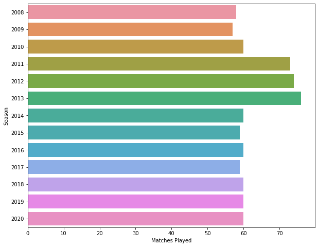
#SEASONWISE MATCHES PLAYED IN IPL
plt.figure(figsize=(10,8))
data = iplm_new.groupby([‘m_id’,’season’]).count().index.droplevel(level=0).value_counts().sort_index()
sns.barplot(y=data.index,x=data,orient=’h’)
plt.xlabel(‘Matches Played’)
plt.ylabel(‘Season’)
plt.show()
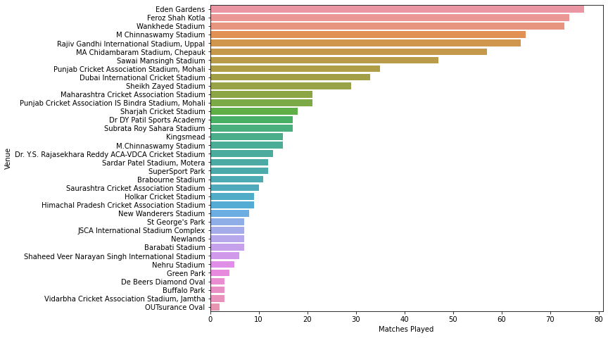
Most IPL Matches by Venue
venues_count=iplm_new.groupby([‘venue’,’m_id’]).count().droplevel(level=1).index.value_counts()
top10_venues =venues_count.head(10)
top10_venues
plt.figure(figsize=(10,8))
data = iplm_new[‘venue’].value_counts().sort_values(ascending=False)
sns.barplot(y=data.index,x=data,orient=’h’)
plt.xlabel(‘Matches Played’)
plt.ylabel(‘Venue’)
plt.show()
batsmanscore_count=iplb_new.groupby([‘batsman’,’batsman_runs’, ‘m_id’]).sum().droplevel(level=1).index.value_counts()
top10_batsmans =batsmanscore_count.head(20)
top10_batsmans
Pivoting the data
df = iplb_new
pd.pivot_table(df,index=[“batsman”])
Top Batsmen of IPL Using Pivot Table
####WHAT IF YOU WANT TO KNOW TO WHICH TEAM THE LEADING BATSMEN BELONG TO?
res_df = pd.pivot_table(df,index=[“batsman”, ‘batting_team’],values=[“batsman_runs”],aggfunc=np.sum)
batsman_score=res_df.sort_values(by=[‘batsman_runs’]) ##by default sort is in ascending if U want descending then set ‘ascending=False’
batsman_score= res_df.sort_values(by=[‘batsman_runs’],ascending=False)
top10_batsman = batsman_score.head(10)
top10_batsman
table = pd.pivot_table(df,index=[“batsman”, ‘batting_team’],columns=[“bowling_team”],values=[“batsman_runs”, “m_id”],
aggfunc={“batsman_runs”:[np.sum]},fill_value=0)
#batsman_score=table.sort_values(by=[‘batsman_runs’]) ##by default sort is in ascending if U want descending then set ‘ascending=False’
batsman_score= table.sort_values(by=[‘batsman’],ascending=True)
batsman_score
result=batsman_score.query(‘batsman == [“V Kohli”]’)
#result=batsman_score.query(‘batsman == [“MS Dhoni”]’)
#result=batsman_score.query(‘batsman == [“Yuvraj Singh”]’)
result
table1 = pd.pivot_table(df,index=[‘batsman’,’bowling_team’],values=[‘batsman_runs’], aggfunc=np.sum)
table1
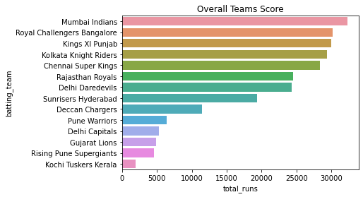
Most Run Scored by IPL Teams
data = iplb_new.groupby([‘batting_team’])[‘total_runs’].sum().sort_values(ascending=False)
data
data = iplb_new.groupby([‘batting_team’])[‘total_runs’].sum().sort_values(ascending=False)
sns.barplot(y=data.index,x=data,orient=’h’)
plt.title(“Overall Teams Score”)
plt.xlabel(‘total_runs’)
plt.ylabel(‘batting_team’)
plt.show()
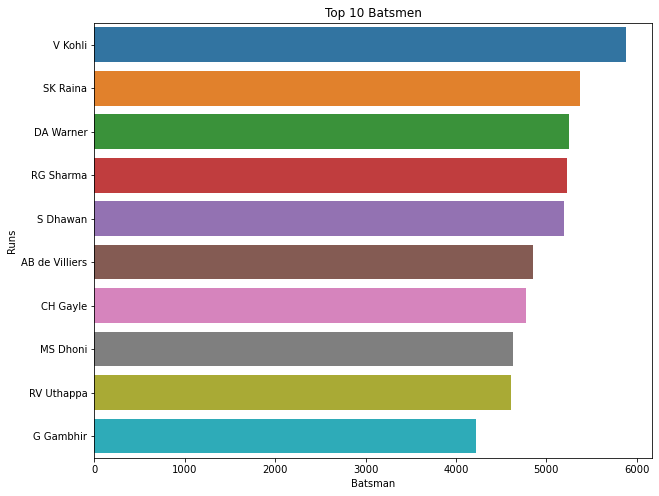
Most Run Scored by Indivdual batsman
iplb_new.groupby([‘batsman’])[‘batsman_runs’].sum().sort_values(ascending=False)[:10]
plt.figure(figsize=(10,8))
data = iplb_new.groupby([‘batsman’])[‘batsman_runs’].sum().sort_values(ascending=False)[:10]
print(type(data))
sns.barplot(y=data.index,x=data,orient=’h’)
plt.title(“Top 10 Batsmen”)
plt.xlabel(‘Batsman’)
plt.ylabel(‘Runs’)
plt.show()
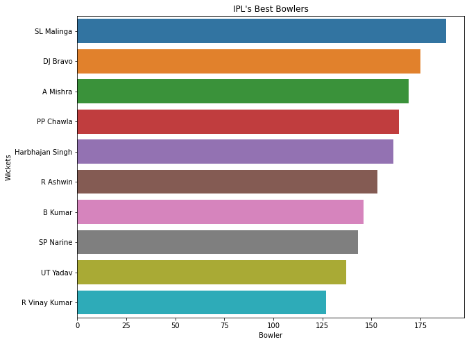
MOST Wickets TAKEN BY Indivdual BOWLER
iplb_new.groupby([‘bowler’])[‘is_wicket’].sum().sort_values(ascending=False)[:10]
plt.figure(figsize=(10,8))
data = iplb_new.groupby([‘bowler’])[‘is_wicket’].sum().sort_values(ascending=False)[:10]
print(type(data))
sns.barplot(y=data.index,x=data,orient=’h’)
plt.title(“IPL’s Best Bowlers”)
plt.xlabel(‘Bowler’)
plt.ylabel(‘Wickets’)
plt.show()
Best Performing Teams in Powerplay
data = iplb_new[iplb_new[‘over’]<6].groupby([‘m_id’,’batting_team’]).sum()[‘total_runs’].groupby(‘batting_team’).mean().sort_values(ascending=False)[:10]
print(data)
sns.barplot(y=data.index,x=data,orient=’h’)
plt.title(“IPL temas performing best during powerplay”)
plt.xlabel(‘team’)
plt.ylabel(‘over’)
plt.show()
“”” Gujarat Lions:51.76, Kochi Tuskers Kerala : 48.57,Sunrisers Hyderabad 47.71 are the top 3 performers in power play”””

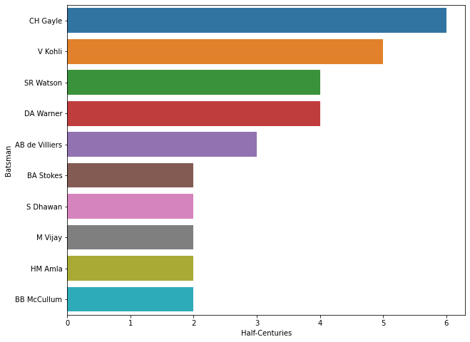
MOST CENTURIES BY IPL PLAYERS
plt.figure(figsize=(10,8))
runs = iplb_new.groupby([‘batsman’,’m_id’])[‘batsman_runs’].sum()
data = runs[runs >= 100].droplevel(level=1).groupby(‘batsman’).count().sort_values(ascending=False)[:10]
print(data)
sns.barplot(y=data.index,x=data,orient=’h’)
plt.xlabel(‘Half-Centuries’)
plt.ylabel(‘Batsman’)
plt.show()
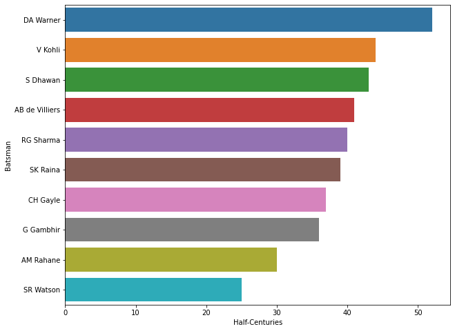
MOST HALF CENTURIES BY IPL PLAYERS
plt.figure(figsize=(10,8))
runs = iplb_new.groupby([‘batsman’,’m_id’])[‘batsman_runs’].sum()
data = runs[runs >= 50].droplevel(level=1).groupby(‘batsman’).count().sort_values(ascending=False)[:10]
print(data)
sns.barplot(y=data.index,x=data,orient=’h’)
plt.xlabel(‘Half-Centuries’)
plt.ylabel(‘Batsman’)
plt.show()
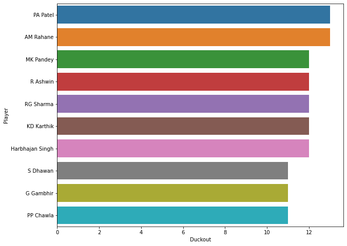
IPL PLAYERS DUCK OUT
plt.figure(figsize=(10,8))
runs = iplb_new.groupby([‘batsman’,’m_id’])[‘batsman_runs’].sum()
data = runs[runs == 0].droplevel(level=1).groupby(‘batsman’).count().sort_values(ascending=False)[:10]
print(data)
sns.barplot(y=data.index,x=data,orient=’h’)
plt.xlabel(‘Duckout’)
plt.ylabel(‘Player’)
plt.show()
Batsman of the Season/Orange Cap
data = iplb_new.groupby([‘season’,’batsman’])[‘batsman_runs’].sum().groupby(‘season’).max()
temp_df=pd.DataFrame(iplb_new.groupby([‘season’,’batsman’])[‘batsman_runs’].sum())
print(“{0:10}{1:20}{2:30}”.format(“Dseason”,”Dbatsman”,”Dscore”))
for season,run in data.items():
player = temp_df.loc[season][temp_df.loc[season][‘batsman_runs’] == run].index[0]
print(season,’\t ‘,player,’\t\t’,run)
Bowler of the Season/Purple Cap
data = iplb_new.groupby([‘season’,’bowler’])[‘is_wicket’].sum().groupby(‘season’).max()
temp_df=pd.DataFrame(df.groupby([‘season’,’bowler’])[‘is_wicket’].sum())
print(“{0:10}{1:20}{2:30}”.format(“Dseason”,”Dbowler”,”Dwickets”))
for season,wicket_taken in data.items():
bowler = temp_df.loc[season][temp_df.loc[season][‘is_wicket’] == wicket_taken].index[0]
print(season,’\t ‘,bowler,’\t\t’,wicket_taken)
Player Hitting Most Sixes in IPL seasons
temp = iplb_new[iplb_new[‘batsman_runs’] == 6].groupby([‘season’,’batsman’]).count()[‘m_id’].sort_values(ascending=False).droplevel(level=0)[:10]
temp
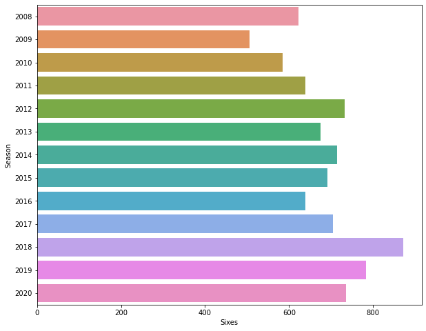
Total sixes in a season
plt.figure(figsize=(10,8))
data = iplb_new[iplb_new[‘batsman_runs’] == 6].groupby(‘season’).count()[‘m_id’].sort_values(ascending=False)
sns.barplot(y=data.index,x=data,orient=’h’)
plt.xlabel(‘Sixes’)
plt.ylabel(‘Season’)
plt.show()
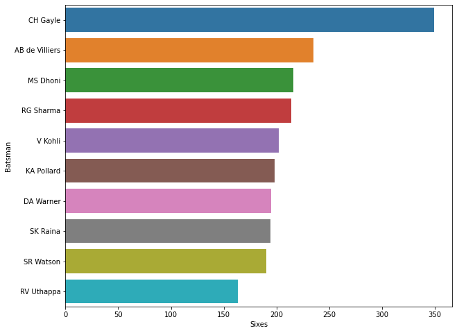
Most IPL Sixes Hit by a batsman
plt.figure(figsize=(10,8))
data = iplb_new[iplb_new[‘batsman_runs’] == 6][‘batsman’].value_counts()[:10]
sns.barplot(y=data.index,x=data,orient=’h’)
plt.xlabel(‘Sixes’)
plt.ylabel(‘Batsman’)
plt.show()
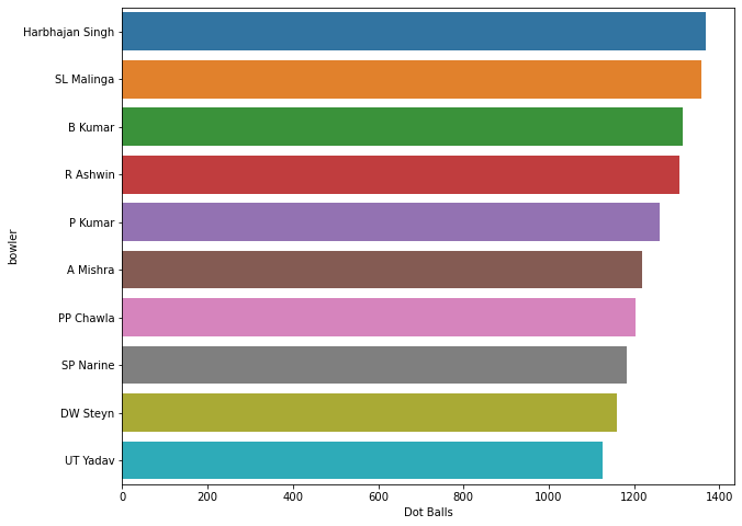
Most dot ball by a bowler
plt.figure(figsize=(10,8))
data = iplb_new[iplb_new[‘batsman_runs’] == 0].groupby(‘bowler’).count()[‘m_id’].sort_values(ascending=False)[:10]
sns.barplot(y=data.index,x=data,orient=’h’)
plt.xlabel(‘Dot Balls’)
plt.ylabel(‘bowler’)
plt.show()
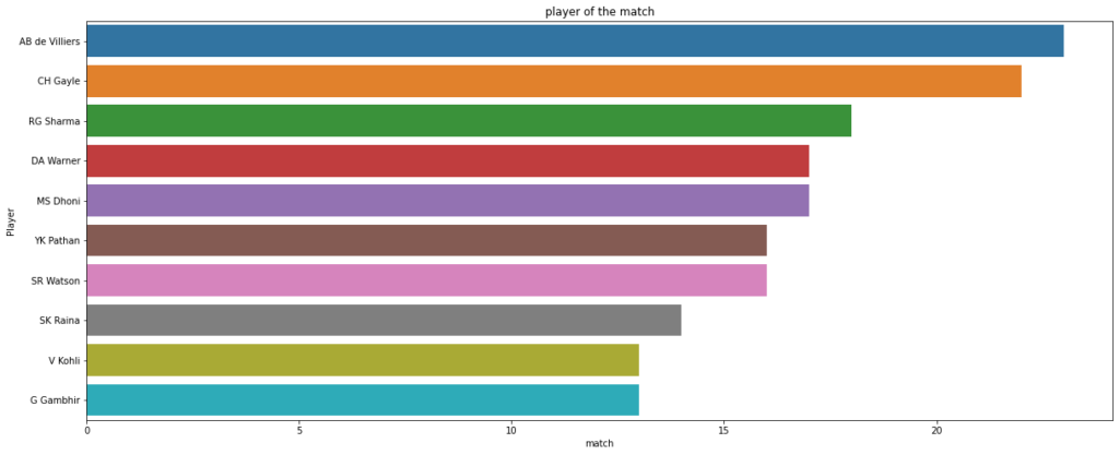
Player of the match Details
plt.figure(figsize=(20,8))
top_players = iplm_new.player_of_match.value_counts()[:10]
#sns.barplot(x=”day”, y=”total_bill”, data=tips)
sns.barplot(y=top_players.index,x=top_players,orient=’h’)
plt.title(“player of the match”)
plt.xlabel(‘match’)
plt.ylabel(‘Player’)
plt.show()
Teamwise Winning Performance
iplm_new[iplm_new[‘result_margin’]>0].groupby([‘winner’])[‘result_margin’].apply(np.mean).sort_values(ascending = False)
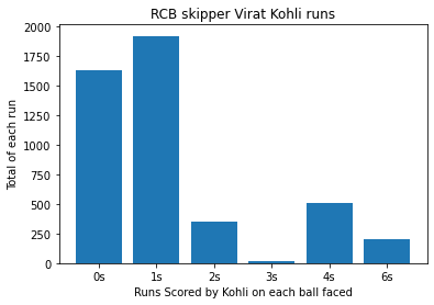
Virat Kohli
# Creating a New Dataframe For Virat Kohli
iplb_kohli = iplb_new[iplb_new[‘batsman’] == “V Kohli”]
iplb_kohli.head(3)
res = iplb[iplb[‘batsman’] ==’V Kohli’]
runs_scored = [res[‘batsman_runs’].sum()]
runs0_scored = res[‘batsman_runs’] == 0
runs1_scored = res[‘batsman_runs’] == 1
runs2_scored = res[‘batsman_runs’] == 2
runs3_scored = res[‘batsman_runs’] == 3
runs4_scored = res[‘batsman_runs’] == 4
runs6_scored = res[‘batsman_runs’] == 6
print(type(runs0_scored))
runs0_scored=runs0_scored.sum()
runs1_scored=runs1_scored.sum()
runs2_scored=runs2_scored.sum()
runs3_scored=runs3_scored.sum()
runs4_scored=runs4_scored.sum()
runs6_scored=runs6_scored.sum()
x = [runs0_scored, runs1_scored, runs2_scored, runs3_scored, runs4_scored, runs6_scored]
y = [0,1,2,3,4,6]
runs1_scored
x1 = [runs0_scored, runs1_scored, runs2_scored, runs3_scored, runs4_scored, runs6_scored]
y1 = [“0s”,”1s”,”2s”,”3s”,”4s”,”6s”]
#plt.plot(y,x)
plt.bar(y1, x1)
plt.xlabel(“Runs Scored by Kohli on each ball faced”)
plt.ylabel(“Total of each run”)
plt.title(“RCB skipper Virat Kohli runs”)
plt.show()