Money Heist

is a Spanish heist crime drama television series created by Álex Pina. The series traces two long-prepared heists led by the Professor (Álvaro Morte), one on the Royal Mint of Spain, and one on the Bank of Spain, told from the perspective of one of the robbers, Tokyo (Úrsula Corberó). The narrative is told in a real-time-like fashion and relies on flashbacks, time-jumps, hidden character motivations, and an unreliable narrator for complexity.

“Money Heist” (“La Casa de Papel”) is a Spanish series.
“Money Heist” is the most in-demand series globally across all platforms, according to Parrot Analytics
IMDB rating: 8.3
Money Heist: Netflix only paid $2 to buy ‘La Casa de Papel’ (assumed earning 365 crores to 401 crores not officially declared)
Season1: $3.0 to 3.3 million
Season2: $4.3 to 7.8 million
Season3: $9 to 9.4 million
Season4: $9.7 to 10.3 million
Season5(partA&partB): $11.1 to 15.7 million
Total budget $46.2 million
Rio: 55000+ Denver: 55000+ inspector Raquel: 6500 +
inspector alisha: 65000 + Helsinki 70000 + Nairobi: 75000, +Tokyo: 100000, + Berlin: 100000, + Professor: 120000)×8
=705,000
Even if the actors get 1% of net profit total earning per episode, for 8episodes series the income will be $564,000,000 fifty-six million four hundred thousand dollars ~ or ~ 38513622416.8 crores ($rate 74.3). 

#Import the following libraries

import pandas as pd
import numpy as np
import matplotlib.pyplot as plt
%matplotlib inline
import seaborn as sns
 

#Loading the data sets

df =  pd.read_excel(“money_heist_all_seasons.xlsx”)
print(df.shape)
df.head()
 

#Creating the word cloud

# importing all necessary modules
from wordcloud import WordCloud, STOPWORDS
import matplotlib.pyplot as plt
import pandas as pd
print(” Money Heist is a Spanish series original namr is (La Casa de Papel) “)
summary_words = “” ###initialized to null
stopwords = set(STOPWORDS)
# iterate through the csv file
for val in df.Summary:
  
  # typecaste each val to string
  val = str(val)
  # split the value
  tokens = val.split()
  
  # Converts each token into lowercase
  for i in range(len(tokens)):
    tokens[i] = tokens[i].lower()
  
  summary_words += ” “.join(tokens)+” “
wordcloud = WordCloud(width = 800, height = 800,
        background_color =’white’,
        stopwords = stopwords,
        min_font_size = 10).generate(summary_words)
# plot the WordCloud image          
plt.figure(figsize = (8, 8), facecolor = None)
plt.imshow(wordcloud)
plt.axis(“off”)
plt.tight_layout(pad = 0)
plt.show()

#Finding the frequency distinct in the tokens

# Importing FreqDist library from nltk and passing token into FreqDist
from nltk.probability import FreqDist
fdist = FreqDist(tokens)
fdist
 

#To find the frequency of top 10 words

fdist1 = fdist.most_common(10)
fdist1
 

#tokens

print(type(fdist))
tokens
print(len(summary_words))
summary_words
 

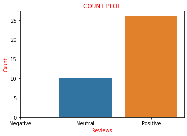
#Finding the sentiments of a sentence

mytext = “jealousy towards mónica and rio”
 

#Extracting only text field

new_df=df[[‘Name’,’Summary’]]
print(“Shape of data=>”,new_df.shape)
new_df.head(5)
 

#Checking whether there are any empty values in data frame

print(new_df.isnull().sum())
new_df.tail(5) #last 5 instances
 

# Displaying the unique names

new_df[“Name”]
print(“unique elements count:”, len(df[“Name”].unique()), “\n”,df[“Name”].unique())
 

#Data Cleaning

for index,text in enumerate(new_df[‘Name’][0:5]):
    print(‘Episode Name %d:\n’%(index+1),text)
for index,text in enumerate(new_df[‘Summary’][0:5]):
    print(‘Episode Summary %d:\n’%(index+1),text)
 

#Expand Contractions

#Contractions are the shortened versions of words like don’t for do not and how’ll for how will etc. We need to expand it.


import re
# Dictionary of English Contractions
contractions_dict = { “ain’t”: “are not”,”‘s”:” is”,”aren’t”: “are not”,
                     “can’t”: “cannot”,”can’t’ve”: “cannot have”,
                     “’cause”: “because”,”could’ve”: “could have”,”couldn’t”: “could not”,
                     “couldn’t’ve”: “could not have”, “didn’t”: “did not”,”doesn’t”: “does not”,
                     “don’t”: “do not”,”hadn’t”: “had not”,”hadn’t’ve”: “had not have”,
                     “hasn’t”: “has not”,”haven’t”: “have not”,”he’d”: “he would”,
                     “he’d’ve”: “he would have”,”he’ll”: “he will”, “he’ll’ve”: “he will have”,
                     “how’d”: “how did”,”how’d’y”: “how do you”,”how’ll”: “how will”,
                     “I’d”: “I would”, “I’d’ve”: “I would have”,”I’ll”: “I will”,
                     “I’ll’ve”: “I will have”,”I’m”: “I am”,”I’ve”: “I have”, “isn’t”: “is not”,
                     “it’d”: “it would”,”it’d’ve”: “it would have”,”it’ll”: “it will”,
                     “it’ll’ve”: “it will have”, “let’s”: “let us”,”ma’am”: “madam”,
                     “mayn’t”: “may not”,”might’ve”: “might have”,”mightn’t”: “might not”, 
                     “mightn’t’ve”: “might not have”,”must’ve”: “must have”,”mustn’t”: “must not”,
                     “mustn’t’ve”: “must not have”, “needn’t”: “need not”,
                     “needn’t’ve”: “need not have”,”o’clock”: “of the clock”,”oughtn’t”: “ought not”,
                     “oughtn’t’ve”: “ought not have”,”shan’t”: “shall not”,”sha’n’t”: “shall not”,
                     “shan’t’ve”: “shall not have”,”she’d”: “she would”,”she’d’ve”: “she would have”,
                     “she’ll”: “she will”, “she’ll’ve”: “she will have”,”should’ve”: “should have”,
                     “shouldn’t”: “should not”, “shouldn’t’ve”: “should not have”,”so’ve”: “so have”,
                     “that’d”: “that would”,”that’d’ve”: “that would have”, “there’d”: “there would”,
                     “there’d’ve”: “there would have”, “they’d”: “they would”,
                     “they’d’ve”: “they would have”,”they’ll”: “they will”,
                     “they’ll’ve”: “they will have”, “they’re”: “they are”,”they’ve”: “they have”,
                     “to’ve”: “to have”,”wasn’t”: “was not”,”we’d”: “we would”,
                     “we’d’ve”: “we would have”,”we’ll”: “we will”,”we’ll’ve”: “we will have”,
                     “we’re”: “we are”,”we’ve”: “we have”, “weren’t”: “were not”,”what’ll”: “what will”,
                     “what’ll’ve”: “what will have”,”what’re”: “what are”, “what’ve”: “what have”,
                     “when’ve”: “when have”,”where’d”: “where did”, “where’ve”: “where have”,
                     “who’ll”: “who will”,”who’ll’ve”: “who will have”,”who’ve”: “who have”,
                     “why’ve”: “why have”,”will’ve”: “will have”,”won’t”: “will not”,
                     “won’t’ve”: “will not have”, “would’ve”: “would have”,”wouldn’t”: “would not”,
                     “wouldn’t’ve”: “would not have”,”y’all”: “you all”, “y’all’d”: “you all would”,
                     “y’all’d’ve”: “you all would have”,”y’all’re”: “you all are”,
                     “y’all’ve”: “you all have”, “you’d”: “you would”,”you’d’ve”: “you would have”,
                     “you’ll”: “you will”,”you’ll’ve”: “you will have”, “you’re”: “you are”,
                     “you’ve”: “you have”}


# Regular expression for finding contractions

contractions_re=re.compile(‘(%s)’ % ‘|’.join(contractions_dict.keys()))


# Function for expanding contractions

def expand_contractions(text,contractions_dict=contractions_dict):
    def replace(match):
        return contractions_dict[match.group(0)]
    return contractions_re.sub(replace, text)


# Expanding Contractions in the reviews and storing as a seperate column

new_df[‘Summary’]=new_df[‘Summary’].apply(lambda x:expand_contractions(x))
new_df.head()

#Store the cleaned reviews in the new column

new_df[‘cleanedSummary’]=new_df[‘Summary’].apply(lambda x:expand_contractions(x))
new_df.head() ###Check the cleaned dataset
 

##Lowercase the reviews

new_df[‘cleanedSummary’]=new_df[‘Summary’].apply(lambda x: x.lower())
new_df.head()
 

#Remove digits and words containing digits

new_df[‘cleanedSummary’]=new_df[‘cleanedSummary’].apply(lambda x: re.sub(‘\w*\d\w*’,”, x))
new_df.head() ####Observe the difference the numbers and number containing words are removed

#Removing Punctuations

# initializing punctuations string
punc = ”’!()-[]{};:'”\,<>./?@#$%^&*_~”’
new_df[‘cleanedSummary’]=new_df[‘cleanedSummary’].apply(lambda x: re.sub(‘[%s]’ % re.escape(punc), ”, x))
new_df.head()
 

#Preparing Text Data for Exploratory Data Analysis (EDA)


#1) Stopwords Removal : Removing the most common words of a language like ‘I’, ‘this’, ‘is’, ‘in’

#2) Lemmatization : reducing a token to its lemma. It uses vocabulary, word structure, part of speech tags, and grammar relations to convert a word to its base form using builtin library like spacy, nltk etc.

#3) Create Document Term Matrix

#Removing Extra Spaces

new_df[‘cleanedSummary’]=new_df[‘cleanedSummary’].apply(lambda x: re.sub(‘ +’,’ ‘,x))
new_df.head()
 
import nltk
nltk.download(“wordnet”)
from nltk.stem import WordNetLemmatizer
 

# Python program to generate WordCloud

# importing all necessary modules
from wordcloud import WordCloud, STOPWORDS
import matplotlib.pyplot as plt
import pandas as pd

print(” Money Heist is a Spanish series original namr is (La Casa de Papel) “)

summary_words = “” ###initialized to null
stopwords = set(STOPWORDS)

# iterate through the csv file
for val in new_df.cleanedSummary:
  
  # typecaste each val to string
  val = str(val)

  # split the value
  tokens = val.split()
  
  # Converts each token into lowercase
  for i in range(len(tokens)):
    tokens[i] = tokens[i].lower()
  
  summary_words += ” “.join(tokens)+” “

wordcloud = WordCloud(width = 800, height = 800,
        background_color =’white’,
        stopwords = stopwords,
        min_font_size = 10).generate(summary_words)

# plot the WordCloud image          
plt.figure(figsize = (8, 8), facecolor = None)
plt.imshow(wordcloud)
plt.axis(“off”)
plt.tight_layout(pad = 0)
plt.show()
lemmatizer = WordNetLemmatizer()
#sentence = “We are putting in the efforts to enhance our understanding of Lemmatization”
tokens = summary_words.split()
print(“tokens :”, tokens)
 
lemmatized_tokens = ” “.join([lemmatizer.lemmatize(token) for token in tokens])
lemmatized_tokens
 

#parts of Speach Tagger

nltk.download(‘averaged_perceptron_tagger’)
pos_tags = nltk.pos_tag(tokens)
pos_tags
from bs4 import BeautifulSoup
a=[]
for i in df[‘IMDB’]:
    if i >8.0:                              
        a.append(1)
    if i==8.0:
        a.append(0)
    if i<8.0:
        a.append(-1)
a
sns.countplot(a)
plt.xlabel(‘Reviews’, color = ‘red’)
plt.ylabel(‘Count’, color = ‘red’)
plt.xticks([-1,0,1],[‘Negative’,’Neutral’,’Positive’])
plt.title(‘COUNT PLOT’, color = ‘r’)
plt.show()

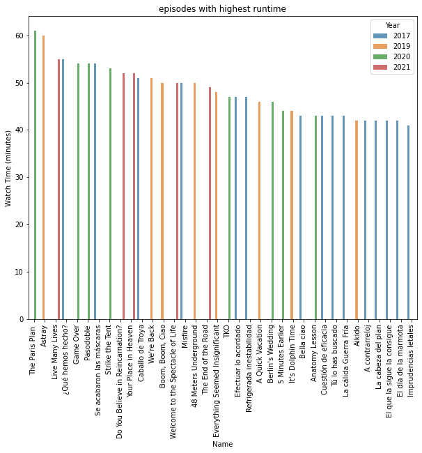
plt.figure(figsize=(10,8))
sns.barplot(x=”Name”,y=”Watch Time (minutes)”,data=df.sort_values(“Watch Time (minutes)”,ascending=False),hue=”Year”,alpha=0.75);plt.xticks(rotation=90)
plt.title(“episodes with highest runtime”);plt.show()


The paris plan episode has longest watchtime

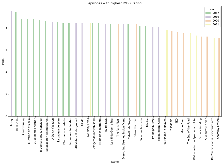
plt.figure(figsize=(15,8))
sns.categorical.barplot(x=”Name”,y=”IMDB”,data=df.sort_values(“IMDB”,ascending=False),hue=”Year”,alpha=0.75,palette=”Accent”);plt.xticks(rotation=90)
plt.title(“episodes with highest IMDB Rating”);plt.show()

Astray episode has highest rating as per Imdb